Usage of py_simple_report
Currently py_simple_report supports
Crosstabulation with stratification
Barplot
Stacked barplot
Crosstabulation for multiple binaries with stratification
Barplot
Heatmap
Dataset
Here, we use Rdataset, “plantTraits” in the statsmodels. Docs of this dataset can be accessed from here.
[1]:
import tqdm
import numpy as np
import pandas as pd
import statsmodels.api as sm
import py_simple_report as sim_repo
[2]:
sim_repo.__version__
[2]:
'0.3.8'
[3]:
df = sm.datasets.get_rdataset("plantTraits", "cluster").data.reset_index()
n = df.shape[0]
print(df.shape)
# Add missing
np.random.seed(1234)
rnd1 = np.random.randint(n, size=6)
cols = ["mycor", "vegsout"]
df.loc[rnd1, cols] = np.nan
(136, 32)
Since we do not have variable table for this dataset, just create. See, items are comma separated and connected via “=” (equal).
[4]:
df_var = pd.DataFrame({
    "var_name": ["mycor", "height", "vegsout", "autopoll", "piq", "ros", "semiros"],
    "description" : ["Mycorrhizas",
                     "Plan height",
                     "underground vegetative propagation",
                     "selfing pollination",
                     "thorny",
                     "rosette",
                     "semiros"
                    ],
    "items" : ["0=never,1=sometimes,2=always",
               np.nan,
               "0=never,1=present but limited,2=important",
               "0=never,1=rare,2=often,3=rule",
               "0=non-thorny,1=thorny",
               "0=non-rosette,1=rosette",
               "0=non-semiros,1=semiros",
              ],
})
[5]:
df_var.head()
[5]:
| var_name | description | items | |
|---|---|---|---|
| 0 | mycor | Mycorrhizas | 0=never,1=sometimes,2=always |
| 1 | height | Plan height | NaN |
| 2 | vegsout | underground vegetative propagation | 0=never,1=present but limited,2=important |
| 3 | autopoll | selfing pollination | 0=never,1=rare,2=often,3=rule |
| 4 | piq | thorny | 0=non-thorny,1=thorny |
QuestionDataContainer
[6]:
# Manually
qdc = sim_repo.QuestionDataContainer(
    var_name="mycor",
    desc="Mycorrhizas",
    title="Mycor",
    missing="missing", # name of missing
    order = ["never", "sometimes", "always"] # used for ordering indexes or columns
)
[7]:
qdc.show() # can access information of QuestionDataContainer
var_name : mycor
desc : Mycorrhizas
title : Mycor
missing : missing
dic : None
order : ['never', 'sometimes', 'always']
[8]:
# From a variable table.
col_var_name = "var_name"
col_item = "items"
col_desc = "description"
qdcs_dic = sim_repo.question_data_containers_from_dataframe(
    df_var, col_var_name, col_item, col_desc, missing="missing")
[9]:
print(qdcs_dic.keys())
dict_keys(['mycor', 'vegsout', 'autopoll', 'piq', 'ros', 'semiros'])
[10]:
qdc = qdcs_dic["mycor"]
qdc.show()
var_name : mycor
desc : Mycorrhizas
title : mycor_Mycorrhizas
missing : missing
dic : OrderedDict([(0.0, 'never'), (1.0, 'sometimes'), (2.0, 'always'), (nan, 'missing')])
order : odict_values(['never', 'sometimes', 'always', 'missing'])
Visualization
Giving two question data container to function producese a graph. From now on, data is always stratified by “autopoll”, the variable name of qdc for “autopoll” is set to be “qdc_strf”
[11]:
qdc1 = qdcs_dic["vegsout"]
qdc_strf = qdcs_dic["autopoll"]
qdc_strf.order = ['never', 'rare', 'often', 'rule'] # not to show "missing"
[12]:
qdc_strf.show()
var_name : autopoll
desc : selfing pollination
title : autopoll_selfing pollination
missing : missing
dic : OrderedDict([(0.0, 'never'), (1.0, 'rare'), (2.0, 'often'), (3.0, 'rule'), (nan, 'missing')])
order : ['never', 'rare', 'often', 'rule']
[13]:
sim_repo.output_crosstab_cate_barplot(
    df,
    qdc1,
    qdc_strf)
| vegsout | never | present but limited | important | missing | All |
|---|---|---|---|---|---|
| autopoll | |||||
| never | 47 | 13 | 8 | 5 | 73 |
| rare | 13 | 3 | 8 | 2 | 26 |
| often | 11 | 3 | 2 | 0 | 16 |
| rule | 20 | 0 | 0 | 1 | 21 |
| All | 91 | 19 | 18 | 8 | 136 |
| vegsout | never | present but limited | important | missing |
|---|---|---|---|---|
| autopoll | ||||
| never | 64.383562 | 17.808219 | 10.958904 | 6.849315 |
| rare | 50.000000 | 11.538462 | 30.769231 | 7.692308 |
| often | 68.750000 | 18.750000 | 12.500000 | 0.000000 |
| rule | 95.238095 | 0.000000 | 0.000000 | 4.761905 |
| All | 66.911765 | 13.970588 | 13.235294 | 5.882353 |
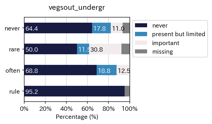

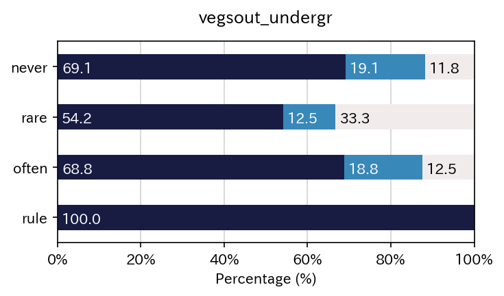
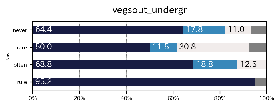
Got it!!
You now see, two tables of cross tabulated data, and three elements of figures. - a simple figure with legend (this can be ugly when label names are too long) - a figure witout legend - only a legend
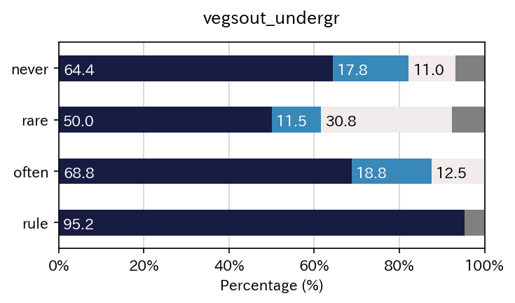
With parameters available.
[14]:
!mkdir test
mkdir: cannot create directory ‘test’: File exists
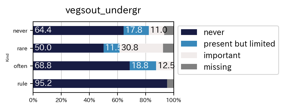
[15]:
dir2save = "./test"
[16]:
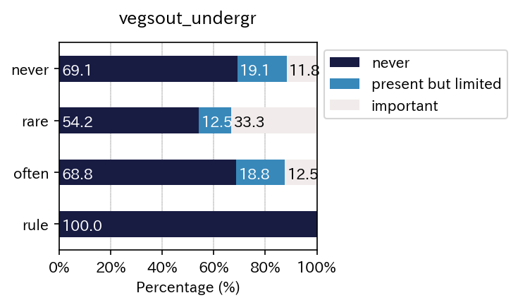
sim_repo.output_crosstab_cate_barplot(
    df,
    qdc1,
    qdc_strf,
    skip_miss=True,
    save_fig_path = dir2save + "/vegsout_undergr.png",
    save_num_path = dir2save + "/number.csv",
    decimal = 4
)
| vegsout | never | present but limited | important | missing | All |
|---|---|---|---|---|---|
| autopoll | |||||
| never | 47 | 13 | 8 | 5 | 73 |
| rare | 13 | 3 | 8 | 2 | 26 |
| often | 11 | 3 | 2 | 0 | 16 |
| rule | 20 | 0 | 0 | 1 | 21 |
| All | 91 | 19 | 18 | 8 | 136 |
| vegsout | never | present but limited | important |
|---|---|---|---|
| autopoll | |||
| never | 69.117647 | 19.117647 | 11.764706 |
| rare | 54.166667 | 12.500000 | 33.333333 |
| often | 68.750000 | 18.750000 | 12.500000 |
| rule | 100.000000 | 0.000000 | 0.000000 |
| All | 71.093750 | 14.843750 | 14.062500 |

Just using for loops enables to output multiple results.
[17]:
lis = ['mycor', 'vegsout', 'piq', 'ros', 'semiros']
for var_name in tqdm.tqdm(lis):
    sim_repo.output_crosstab_cate_barplot(
        df,
        qdcs_dic[var_name],
        qdc_strf,
        skip_miss=False,
        save_fig_path = dir2save + f"/{var_name}.png",
        save_num_path = dir2save + "number.csv", # save the number to the same file.
        show=False,
    )
100%|██████████| 5/5 [00:03<00:00, 1.58it/s]
Barplot
Simple barplot version
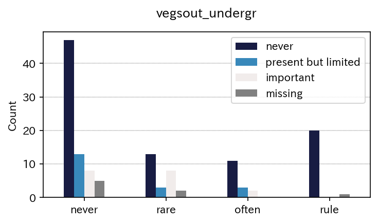
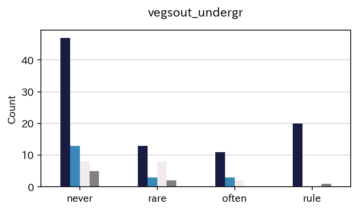
[18]:
sim_repo.output_crosstab_cate_barplot(
    df,qdc_strf, qdc1,  percentage=False, skip_miss=False, stacked=False,  transpose=True
)
| vegsout | never | present but limited | important | missing | All |
|---|---|---|---|---|---|
| autopoll | |||||
| never | 47 | 13 | 8 | 5 | 73 |
| rare | 13 | 3 | 8 | 2 | 26 |
| often | 11 | 3 | 2 | 0 | 16 |
| rule | 20 | 0 | 0 | 1 | 21 |
| All | 91 | 19 | 18 | 8 | 136 |
| vegsout | never | present but limited | important | missing | All |
|---|---|---|---|---|---|
| autopoll | |||||
| never | 47 | 13 | 8 | 5 | 73 |
| rare | 13 | 3 | 8 | 2 | 26 |
| often | 11 | 3 | 2 | 0 | 16 |
| rule | 20 | 0 | 0 | 1 | 21 |
| All | 91 | 19 | 18 | 8 | 136 |

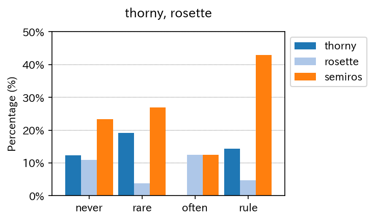
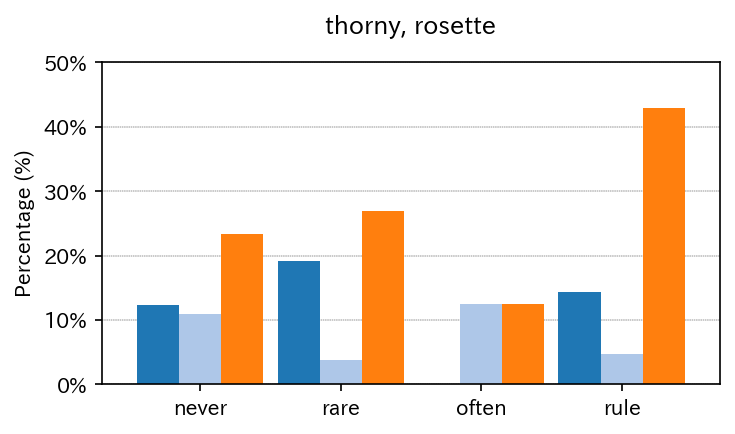
Multiple binaries can be summarized in a single figure.
[19]:
lis = ["piq", "ros", "semiros"]  # variable names
vis_var = sim_repo.VisVariables(ylim=[0,50], cmap_name="tab20", cmap_type="matplotlib")
sim_repo.output_multi_binaries_with_strat(df, lis, qdcs_dic, qdc_strf, vis_var)
| thorny | rosette | semiros | |
|---|---|---|---|
| never | 9 | 8 | 17 |
| rare | 5 | 1 | 7 |
| often | 0 | 2 | 2 |
| rule | 3 | 1 | 9 |
| thorny | rosette | semiros | |
|---|---|---|---|
| never | 12.328767 | 10.958904 | 23.287671 |
| rare | 19.230769 | 3.846154 | 26.923077 |
| often | 0.000000 | 12.500000 | 12.500000 |
| rule | 14.285714 | 4.761905 | 42.857143 |
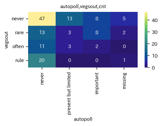
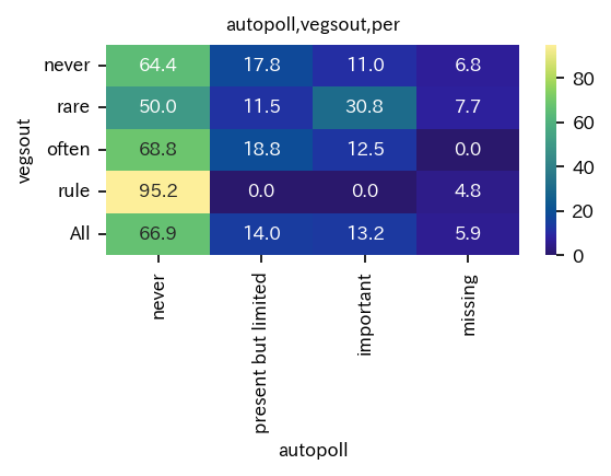
Heatmap
Heatmap of crosstabulation.
[20]:
sim_repo.heatmap_crosstab_from_df(df, qdc_strf, qdc1, xlabel=qdc_strf.var_name, ylabel=qdc1.var_name ,
                                  save_fig_path=dir2save + f"/{qdc_strf.var_name}_{qdc1.var_name}_cnt.png" )
sim_repo.heatmap_crosstab_from_df(df, qdc_strf, qdc1, xlabel=qdc_strf.var_name, ylabel=qdc1.var_name,
                                  normalize="index")
VisVariables
Important classes in py_simple_report is a VisVariables. It controls a figure setting via it values.
[21]:
vis_var = sim_repo.VisVariables(
    figsize=(5,2),
    dpi=200,
    xlabel="",
    ylabel="Kind",
    ylabelsize=5,
    yticksize=7,
    xticksize=7,
)
sim_repo.output_crosstab_cate_barplot(
    df,
    qdc1,
    qdc_strf,
    vis_var = vis_var,
    save_fig_path = dir2save + "/vegsout_undergr_vis_var.png",
    save_num_path = dir2save + "number.csv",
)
| vegsout | never | present but limited | important | missing | All |
|---|---|---|---|---|---|
| autopoll | |||||
| never | 47 | 13 | 8 | 5 | 73 |
| rare | 13 | 3 | 8 | 2 | 26 |
| often | 11 | 3 | 2 | 0 | 16 |
| rule | 20 | 0 | 0 | 1 | 21 |
| All | 91 | 19 | 18 | 8 | 136 |
| vegsout | never | present but limited | important | missing |
|---|---|---|---|---|
| autopoll | ||||
| never | 64.383562 | 17.808219 | 10.958904 | 6.849315 |
| rare | 50.000000 | 11.538462 | 30.769231 | 7.692308 |
| often | 68.750000 | 18.750000 | 12.500000 | 0.000000 |
| rule | 95.238095 | 0.000000 | 0.000000 | 4.761905 |
| All | 66.911765 | 13.970588 | 13.235294 | 5.882353 |

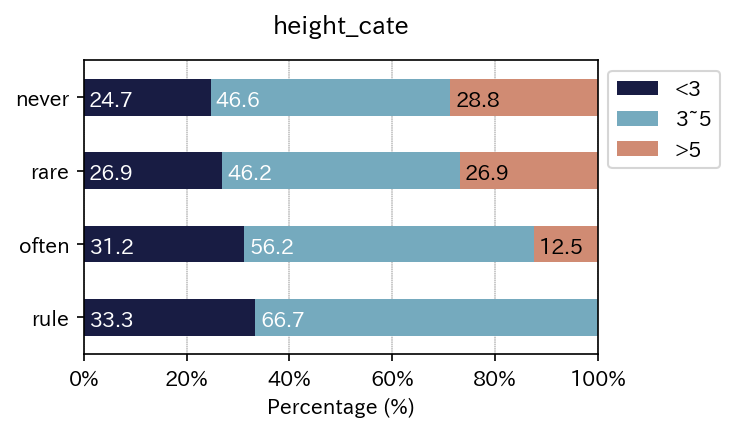
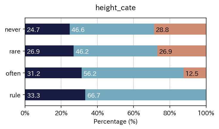
Engineered columns
Of course, engineered columns can be used.
[22]:
height_cate = "height_cate"
ser = df["height"]
df[height_cate] = (ser
                   .mask( ser <= 9, ">5")
                   .mask( ser <= 5, "3~5")
                   .mask( ser < 3 , "<3")
                  )
print(df[height_cate].value_counts())
qdc = sim_repo.QuestionDataContainer(
    var_name=height_cate, order=["<3","3~5",">5"], missing="missing", title=height_cate
)

vis_var = sim_repo.VisVariables()
sim_repo.output_crosstab_cate_barplot(
    df,
    qdc=qdc,
    qdc_strf=qdc_strf,
    show=True,
    vis_var=vis_var,
)
3~5    69
<3     37
>5     30
Name: height_cate, dtype: int64
| height_cate | <3 | 3~5 | >5 | All |
|---|---|---|---|---|
| autopoll | ||||
| never | 18 | 34 | 21 | 73 |
| rare | 7 | 12 | 7 | 26 |
| often | 5 | 9 | 2 | 16 |
| rule | 7 | 14 | 0 | 21 |
| All | 37 | 69 | 30 | 136 |
| height_cate | <3 | 3~5 | >5 |
|---|---|---|---|
| autopoll | |||
| never | 24.657534 | 46.575342 | 28.767123 |
| rare | 26.923077 | 46.153846 | 26.923077 |
| often | 31.250000 | 56.250000 | 12.500000 |
| rule | 33.333333 | 66.666667 | 0.000000 |
| All | 27.205882 | 50.735294 | 22.058824 |