Quickstart
SIR model is used for an example. Explanation of SIR model can be found here.
First, import a module.
[1]:
import matplotlib.pyplot as plt
import py_compart_model as pcm
Prepare parameters for SIR model.
[2]:
R0 = 2
gamma = 1/10
N = 100
beta = R0*gamma/N
Set parameters and compartment model with values or without values. Model definition should be defined inside a context manager, but you can specify initial values for each compartment and values for parameters outside a context manager.
[3]:
_beta  = pcm.Param("beta")
_gamma = pcm.Param("gamma", value=gamma)
with pcm.Model() as m:
    S = m.C("S")
    I = m.C("I")
    R = m.C("R", value=0)
    S.d = - _beta * S * I
    I.d = + _beta * S * I - _gamma * I
    R.d = + _gamma * I
Pass parameters to the model, and create a function for fitting. Currently, py_compart_model takes approch to generate string form of function and execute this string to create function. Since pure function is applied, there is no overhead for calculation for this package.
[4]:
m.create_function((_beta,_gamma))
def _f(t, y, beta, gamma):
    S = y[0]
    I = y[1]
    R = y[2]
    dS =  - beta * (S) * (I)
    dI =  + beta * (S) * (I) - gamma * (I)
    dR =  + gamma * (I)
    return [dS,dI,dR]
Values for parameters and initial values for compartments can be specified after create_function method. This allows us to simulate a model, varying parameters and initial values.
[5]:
_beta.set_value(beta)
S.set_init(N-1)
I.set_init(1)
Then, solve equation. At present, solve uses solve_ivp implemented in scipy. kargs is passed to solve_ivp function.
[6]:
ode_res = m.solve([0,200], max_step=0.1)
Summary print out inits, args and message for solving results.
[7]:
ode_res.summary()
inits : {'S': 99, 'I': 1, 'R': 0}
args : {'beta': 0.002, 'gamma': 0.1}
message : The solver successfully reached the end of the integration interval.
Can access to results of solve_ivp, and results of y are mapped to its variables.
[8]:
res = ode_res.result
print(res)
print(res.I)
        I: array([1.        , 1.00138615, 1.0112454 , ..., 0.003735  , 0.00371264,
       0.00369355])
        R: array([0.00000000e+00, 1.41447896e-03, 1.14775596e-02, ...,
       8.00141757e+01, 8.00142130e+01, 8.00142448e+01])
        S: array([99.        , 98.99719937, 98.97727704, ..., 19.98208926,
       19.98207438, 19.98206167])
  message: 'The solver successfully reached the end of the integration interval.'
     nfev: 12008
     njev: 0
      nlu: 0
      sol: None
   status: 0
  success: True
        t: array([0.00000000e+00, 1.41349951e-02, 1.14134995e-01, ...,
       1.99814135e+02, 1.99914135e+02, 2.00000000e+02])
 t_events: None
        y: array([[9.90000000e+01, 9.89971994e+01, 9.89772770e+01, ...,
        1.99820893e+01, 1.99820744e+01, 1.99820617e+01],
       [1.00000000e+00, 1.00138615e+00, 1.01124540e+00, ...,
        3.73499825e-03, 3.71264206e-03, 3.69355271e-03],
       [0.00000000e+00, 1.41447896e-03, 1.14775596e-02, ...,
        8.00141757e+01, 8.00142130e+01, 8.00142448e+01]])
 y_events: None
[1.         1.00138615 1.0112454  ... 0.003735   0.00371264 0.00369355]
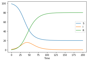
For visualization.
[9]:
pcm.plot_over_time(ode_res)
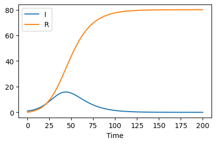
you can pass ax to control visualization and specify both compartment by sting or Compartments class used in contextmanager for plotting.
[10]:
fig = plt.figure(figsize=(5,3),dpi=100)
ax = fig.add_subplot(111)
pcm.plot_over_time(ode_res, comparts=["I", R], ax=ax)
Note
Since this package is not mature, it does not support - Matrix arguments, specify size for each compoment to include stratified simulation. - Does not gurantee no weired behaviors. I can not cover all problems caused from string generated functions.
If you want to improve it, please help me to develop a better one!!
Motivation
If you want to use solve_ivp, you should concatate variables into one. This task is redundunt and causes mistakes. If you want to implement the same SIR model described in Quickstart, code becomes like,
[11]:
from scipy.integrate import solve_ivp
[12]:
def sir(t,y,beta, gamma):
    S = y[0]
    I = y[1]
    R = y[2]
    dS = - beta * S * I
    dI = + beta * S * I - gamma*I
    dR = + gamma*I
    d = [dS,dI,dR]
    return d

R0 = 2
gamma = 1/10
N = 100
beta = R0*gamma/N
res = solve_ivp(sir, [0,200], [N - 1,1,0], args=(beta, gamma),  max_step=0.1)