Usage of contextplt
Contextplt is for writing matplotlib very simply using context manager. This package is a simple wrapper for matplotlib and calls various functions from parameters of context managers.
Quickstart
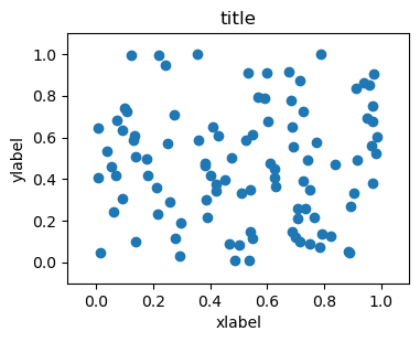
When two dimensional variables are visualized with customized settings, we often use object-based inference instead of pyplot interface like this.
[1]:
import matplotlib.pyplot as plt
import numpy as np

import contextplt as cplt
print(cplt.__version__)
0.2.11
[2]:
x = np.random.random(size=100)
y = np.random.random(size=100)
[3]:
fig = plt.figure(figsize=(4,3), dpi=100)
ax = fig.add_subplot(111)
ax.scatter(x,y)
ax.set_xlabel("xlabel")
ax.set_ylabel("ylabel")
ax.set_xlim([-0.1,1.1])
ax.set_ylim([-0.1,1.1])
plt.title("title")
[3]:
Text(0.5, 1.0, 'title')
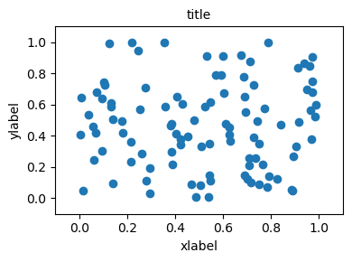
[4]:
with cplt.Single(xlim=[-0.1,1.1], ylim=[-0.1,1.1], xlabel="xlabel", ylabel="ylabel",
        title="title", figsize=(4,3), dpi=100) as p:
    p.ax.scatter(x,y)

[5]:
kargs = dict(xlim=[-0.1,1.1], ylim=[-0.1,1.1], xlabel="xlabel", ylabel="ylabel",
        title="title", figsize=(4,3), dpi=100)
with cplt.Single(**kargs) as p:
    p.ax.scatter(x,y)

x2 = np.random.random(size=100)*0.8
y2 = np.random.random(size=100)*0.8

with cplt.Single(**kargs) as p:
    p.ax.scatter(x2,y2)
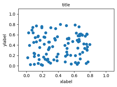
This usage is helpful when figure setting are shared but variables are replaced with new ones.
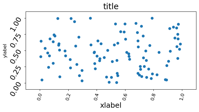
Parameters for cplt.Single
This section explains how to use parameters in cplt.Single. This is a full parameters currently impelemented in cplt.Single.
[6]:
with cplt.Single(
    xlim=[-0.1,1.1],
    ylim=[-0.1,1.1],
    xlabel="xlabel",
    ylabel="ylabel",
    xlabelfontsize=18,
    ylabelfontsize=12,
    xtickfontsize=12,
    ytickfontsize=18,
    title="title",
    titlefontsize=20,
    tight=True,
    xrotation=75,
    yrotation=60,
    save_path="./test.png",
    savefig_kargs=dict(
        facecolor="white", bbox_inches="tight",
    ),
    figsize=(7,4),
    dpi=100,
) as p:
    p.ax.scatter(x,y)
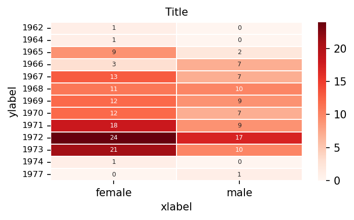
Pandas integration
Since pandas’ plot method accepts ax object, pass p.ax returned by context manager yield a customized figure.
[7]:
import pandas as pd
import seaborn as sns
import statsmodels.api as sm
[8]:
df = sm.datasets.get_rdataset("Melanoma", "MASS").data
df["sex"] = df["sex"].replace({0:"female", 1:"male"})
df_ht = pd.crosstab(df["year"], df["sex"])
[9]:
with cplt.Single(title="Title", xlabel="xlabel", ylabel="ylabel", ytickfontsize=8) as p:
    sns.heatmap(df_ht, cmap="Reds", fmt=".0f", ax=p.ax,
                        annot=True, linewidths=.2, annot_kws={"fontsize":6})
cplt.Multiple
[10]:
x1, x2, y1, y2= np.random.rand(4, 100)
with cplt.Multiple(grid=(2,1),figsize=(5,4), dpi=150) as mul:
    with mul.Single(index=1 ) as p:
        p.ax.scatter(x1,y1)
    with mul.Single(index=2,) as p:
        p.ax.scatter(x2,y2)
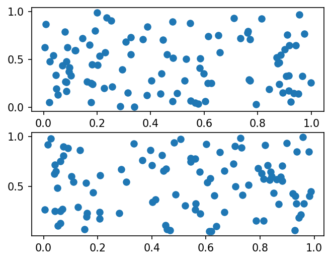
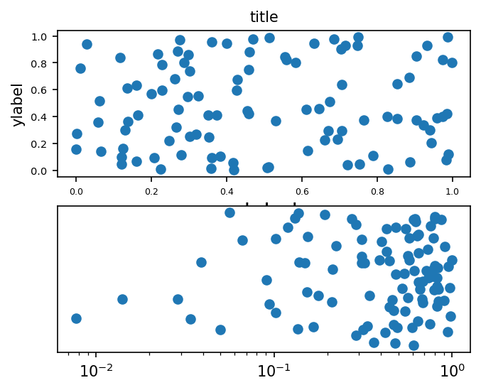
This type of writing is a bit redundant, but it gurantees all of your figures are correctly drawn. Same as cplt.Single, we can use various parameters to control figures.
[11]:
x1, x2, y1, y2= np.random.rand(4, 100)
with cplt.Multiple(grid=(2,1),figsize=(5,4), dpi=150) as mul:
    with mul.Single(index=1 ,
                        xlabel="xlabel", ylabel="ylabel", title="title",
                        xtickfontsize=6, ytickfontsize=7, xlabelfontsize=15) as p:
        p.ax.scatter(x1,y1)
    with mul.Single(index=2,xscale="log", yticks_show=False) as p:
        p.ax.scatter(x2,y2)
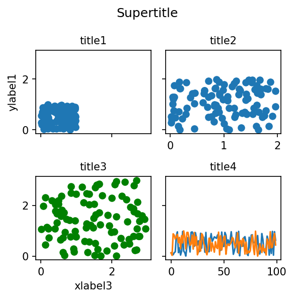
Also, sharex and sharey works as sharing x/y axis between figures. Since ax information is required when drawing next, names returned by context manger should be modified a little.
[12]:
x1, y1 = np.random.rand(2,100)
x2, y2 = np.random.rand(2,100)*2
x3, y3 = np.random.rand(2,100)*3
df = pd.DataFrame(dict(x1=x1,y1=y1))
with cplt.Multiple(grid=(2,2),figsize=(4,4), dpi=150, suptitle="Supertitle", tight=True) as mul:
    with mul.Single(index=1, title="title1", xlabel="xlabel1", ylabel="ylabel1") as p1:
        p1.ax.scatter(x1,y1)
    with mul.Single(index=2, sharey=p1.ax,title="title2") as p2:
        p2.ax.scatter(x2,y2)
    with mul.Single(index=3, sharex=p1.ax, sharey=p1.ax, title="title3", xlabel="xlabel3") as p3:
        p3.ax.scatter(x3,y3, color="green")
    with mul.Single(index=4, sharey=p1.ax, title="title4") as p4:
        df.plot(ax=p4.ax)
        p4.ax.get_legend().set_visible(False)
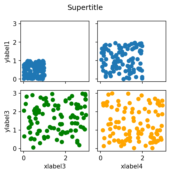
“label_outer” parameter leaves all of the outer information and remove all the inner labels and ticks. Be careful when using it because it also removes inner ticks although ticks are even not shared correctly.
[13]:
x1, y1 = np.random.rand(2,100)
x2, y2 = np.random.rand(2,100)*2
x3, y3 = np.random.rand(2,100)*3
x4, y4 = np.random.rand(2,100)*3
with cplt.Multiple(grid=(2,2),figsize=(4,4), dpi=150, suptitle="Supertitle", tight=True, label_outer=True) as mul:
    with mul.Single(index=1, ylabel="ylabel1", ) as p1:
        p1.ax.scatter(x1,y1)
    with mul.Single(index=2, sharex=p1.ax, sharey=p1.ax) as p2:
        p2.ax.scatter(x2,y2)
    with mul.Single(index=3, sharex=p1.ax, sharey=p1.ax, xlabel="xlabel3", ylabel="ylabel3") as p3:
        p3.ax.scatter(x3,y3, color="green")
    with mul.Single(index=4, sharex=p1.ax, sharey=p1.ax, xlabel="xlabel4") as p4:
        p4.ax.scatter(x4,y4, color="orange")
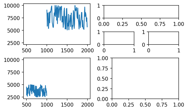
Mosaic plot
[14]:
import contextplt as cplt
x1 = np.arange(1000, 2000, 10)
y1 = np.random.randint(low=5000, high=10000, size=x1.shape)
mosaic = [
    ['A', [['B', 'B'],
           ['D', 'E']]],
    ['F', 'G'],
]
with cplt.Multiple(mosaic = mosaic, sharex=False) as mul:
    with mul.Single(index="A") as p1:
        p1.ax.plot(x1,y1)
    with mul.Single(index="F", sharex=p1.ax, sharey=p1.ax) as p2:
        p2.ax.plot(x1*0.5,y1*0.5)
[ ]: